A problem in two parts


Taken from the VNNCOMP 2021 benchmarks
The verification
Loading diagram...
The goal is to linear the output layer of the neural network and verify the constraints
Common activation functions
Loading diagram...
Loading diagram...
Other notable activation functions
Loading diagram...
Loading diagram...
Linearize the activation functions
The approach used by , winner of VNNCOMP 2021, 2022 and 2023 is to linearize the activation functions, reducing the error introduced by the approximation with tunable parameters.
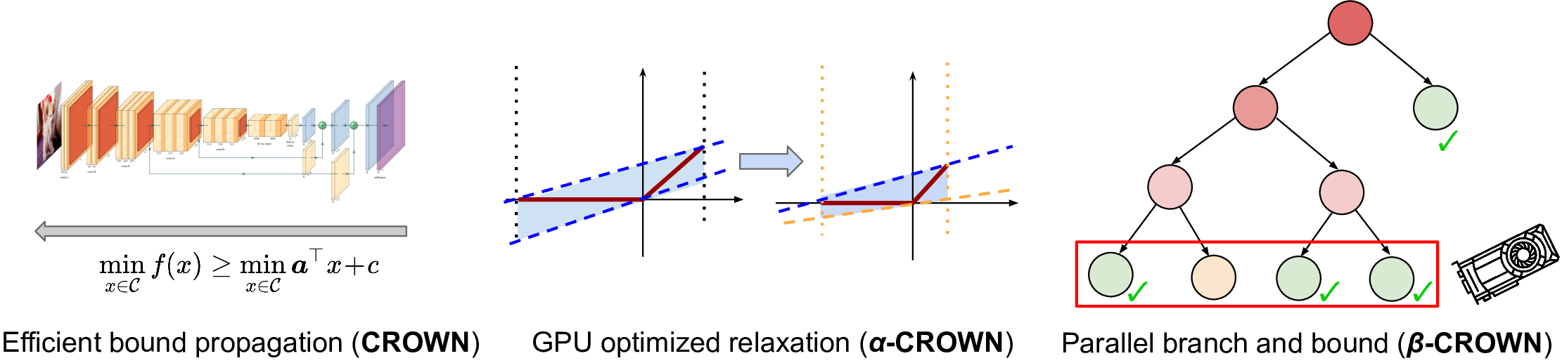
Convex relaxation of Neural Networks
To deal with intractability, convex relaxations can be used. For instance, Planet relaxation substitutes the ReLU function with
where and are the lower and upper bounds of the input . They can be obtained directly or estimated.
Propagate bounds
Bound propagation is a key step in guiding the search for a solution. State-of-the-art tools include LiPRA and PRIMA.
dlinear's current naive implementation only propagate explicit bounds and equality constraints.
These functionalities can be extended by considering the interval bounds of the input variables and propagating them through the graph of constraints.
Sum of infeasibilities
Comparison
| Tool | Strict constraints | Output eq | Correlated inputs | Unbounded | Or | Precision | Efficient |
|---|---|---|---|---|---|---|---|
| dlinear | |||||||
| alpha-beta-crown | * | ||||||
| neurosat | |||||||
| nnenum | |||||||
| Marabou |
SMT components: Terms and formulae
- : propositional variables (Formula)
- : real-valued variables (Term)
- : constants (Term)
- : comparison operators
Conjunctive normal form
Most SMT solvers expect the input in CNF form, where are literals
If-then-else terms
If are formulas, is a formula equivalent to
If are terms and is a formula, is a term
Piecewise linear functions to ITE
Piecewise linear functions can be represented using if-then-else terms
; ReLU
(declare-const x Real)
(declare-const y Real)

(assert (= y (ite (<= x 0) 0 x)))
ITE to CNF
The if-then-else term can be converted to CNF by introducing a fresh variable with the following equisatisfability relation
e.g.
Max encoding
The max function can be seen as a special case of an ITE term. Exploiting its characteristics, introducing two fresh variables allows to encode it directly in CNF:
Linear layers, non-linear activation layers
Given a neural network with layers, we can divide them into two categories:
- Linear layers:
- Input: , weights: , bias:
- Activation layers: non-linear
- Piece-wise linear functions
- General non-linear functions

Tightening the bounds
Converting all the layers of a neural network up to an activation layer to a linear constraint allows to compute the bounds of the output of the activation layer, as long the input is bounded.
Fixing the piecewise linear functions
If the bounds on output of the activation layer are strict enough, it may be possible to fix the piecewise linear term.
Sum of Infeasibilities
Instead of adding the non-fixed activation layers to the constraints of the LP problem, they can be used to minimize the sum of infeasibilities.
Sorting by the violation they introduce gives us a way to prioritize the search for the solution.
Completeness vs Real world
SMT solvers aim for a complete approach, a mathematical solution of the problem, employing symbolic representation of the inputs and exact arithmetic (when possible).
In the real world, however, speed of the computation is usually the main concert, hence floating point arithmetic is almost always used.
As a result, it can happen that the solution found by the SMT solver is not the same as the one computed by the neural network (e.g. OnnxRuntime).
Future work
- Benchmarks
- Other heuristics to optimize the search for the solution
- use overapproximation of bounds to reduce the search space
- How much completeness are we sacrificing?
References
- Symbolic representation with focus on ITE and max terms
- Efficient Term-ITE Conversion for Satisfiability Modulo Theories
- Different approaches to optimize the solution search in the exponential subproblem tree
- Floating-Point Verification using Theorem Proving