Verified Linear Programming through Tolerance-Aware Precision Boosting




E. Casablanca
M. Sidaway
P. Zuliani
S. Soudjani





VSTTE 2026
Bits of computer architecture
Computers use bits to store data, including numbers.
Floating point
Rationals
We only have a finite number of bits.
Motivation
Standard linear program (LP)
with , , .
- Linear Programming is a core component of:
- Optimization
- SMT Solving
- Program Analysis
- Numerical errors undermine soundness.
- Commercial floating-point LP solvers can produce incorrect results.
Solutions
- Rational arithmetic
- Easy to implement, exactness guarantee.
- Slow and memory-intensive.
- Iterative refinement (SoPlex)
- Generally faster.
- Can struggle with numerical issues.
- Precision boosting (QSopt_ex)
- Can solve difficult LPs.
- Limited theoretical justification.
[1] A. Gleixner, D. Steffy, K. Wolter (2016), Iterative Refinement for Linear Programming
[2] D. L. Applegate, W. Cook, S. Dash, D. G. Espinoza (2009), QSopt_ex Rational LP Solver
Goal
Loading diagram...
IEEE 754 Standard
Modern computers implement the IEEE 754 standard for floating-point arithmetic.
where is the base, is the precision, is the integer significand and is the exponent.
Loading diagram...
Operations with floating-point numbers
The IEEE 754 standard provides the following guarantees for floating-point operations:
where is the unit roundoff ( for double precision) and is the floating-point computation of .
Any operation can introduce an error.
Error analysis
Error analysis is the study of how floating-point computations affect our results.
Forward error analysis VS Backward error analysis.
[4] N. J. Higham (2002), Accuracy and Stability of Numerical Algorithms
Ensuring backward stability in the simplex
Given an initial sequence of indices corresponding to the columns of , at each iteration:
- Construct the basis:
- Compute primal vector:
- Compute dual vector:
- Evaluate reduced costs:
- Determine entering variable.
- Determine leaving variable: .
- Pivot and update basis.
Bartels-Golub update
After the initial decomposition of , the factor is updated:
[5] R. H. Bartels (1971), A Stabilization of the Simplex Method
Error analysis
In the backward-error analysis formulation,
we find that
As long as the number of iterations is limited, the backward error is reasonably bounded.
Variable precision floating-point simplex
Loading diagram...
Characteristic constants
For a given input , , and , we can define the following constants:
- is the maximum negative across all reduced costs;
- is the minimum positive element across all s;
- is the smallest difference between the two smallest distinct values of across all bases.
Computing them directly would require exploring all the possible bases.
Convergence of precision boosting
If and hold, then the floating-point simplex makes the same decisions as the exact rational simplex.
Delta-optimality
Theorem
Given , a -complete LP algorithm returns exactly one of the following:
- -optimal: iff it produces a -optimal certificate such that ;
- infeasible: iff the LP is infeasible;
- unbounded: iff the LP is unbounded.
If , then the algorithm is exact.
Precision boosting simplex
Loading diagram...
Delpi
- Delta-complete Exact Linear ProgrammIng framework:
Delpi. - C++ library with python interface.
QSopt_exas a basis.- Implements the -complete procedure.
- Can interface with
SoPlex.
Results
- Sloane–Stufken benchmarks.
- Dense and feasible.
- Numerically challenging.
- Incorrect results from FP SOTA solvers.
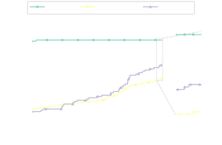
- Performance profile plot.
Future Work
- Integration into SMT solvers (work in progress!)
- Stronger practical heuristics for choosing tolerances
- Extensions to MILP
References
- IEEE (2019) IEEE Standard for Floating-Point Arithmetic
- R. H. Bartels (1971), A Stabilization of the Simplex Method
- N. J. Higham (2002), Accuracy and Stability of Numerical Algorithms
- D. L. Applegate, W. Cook, S. Dash, D. G. Espinoza (2007), Exact Solutions to Linear Programming Problems
- R. Wunderling (1996), Paralleler und objektorientierter simplex-algorithmusr
- A. Gleixner, D. Steffy, K. Wolter (2016), Iterative Refinement for Linear Programming
- A. Gleixner, D. Steffy (2019), Limited-Precision LP Oracles
- L. Eifler, J. Nicolas-Thouvenin, A. Gleixner (2024), Combining Precision Boosting with LP Iterative Refinement
- N. J. A. Sloane, J. Stufken (1996), A linear programming bound for orthogonal arrays with mixed levels
- D. L. Applegate, W. Cook, S. Dash, D. G. Espinoza (2009), QSopt_ex Rational LP Solver